Using LEDs to measure narrow spectral bands of light.
LEDs can be used to measure spectrally narrow bands of light by connecting them to a high-impedance current-to-voltage amplifier and treating them like inefficient photodiodes.
Using LEDs to measure spectrally narrow bands of light
There’s a great deal you can learn about the world around you if you can measure the intensity of light in narrow spectral bands.
Aerosols and ozone in the atmosphere, vegetation and water-stress in terrestrial plants when measured from planes or satelites.
Often narrow spectral bands of light are measured with interference filters. These are optical filters that consist of multiple layers of dielectric materials with different refractive indices and different thicknesses. Interference filters can have bandwidths as low as 10 nm however the construction is complex and a narrow bandwidth filter might need up to 100 layers which means they are expensive.
For example a 25 mm diameter interference filter with a 550 nm bandpass wavelength and a 15 nm bandwidth (FWHM) is about $325: Chroma, ET550/15m
Forrest Mimms pioneered the use of light-emitting-diodes as spectrally selective light detectors for sun photometry in 1992. It turns out that LEDs which normally are used to emit light can also be used to measure light. A very basic green LED from Radio Shack (part# 276-022A) might generate as much as 10 nA of current.
A number of years ago Optometrics let me use some of the equipment they make to test LEDs for their spectral response.
I used their SDMC1-3 300-800 nm scanning digital monochrometer and a 20W tungsten lamp model 7-1110 similar to this current product 20W Tungsten Halogen LKight Source/
Optometrics supplied a calibration for the output of their tungsten light source and a spectral sensitivity the monochrometer which I combined topgether into a variable I called Monochrometer Output Power (uW).
We developed a circuit board with a dual opamp to first convert the tiny currents produced by the LEDs to a voltage and then to amplify the voltage.
At the time I only had a chance to measure two LEDs.
- Green LED, Radio Shack part# 276-022A, 6.3 mcd
- High brightness red LED, Radio Shack part# 276-066B, 470 mcd
The results are impressive – especially for the low-brightness green LED which has a peak response at 550 nm and a bandwidth of 60 nm. While the bandwidth is about four times as wide as the Chroma, ET550/15m interference filter the cost is lower by about a factor of 1000.
The red LED is a high-brightness model and about 75 times brighter than the green LED when used to emit light. However when used as a light sensor the green LED has a narrower bandwidth.
It is easy to see the longer response tail in the shorter wavelengths for the red LED when the same spectral response data is plotted using a log scale on the Y axis. LEDs used as sensors like the green LED with very strong rejection of out of band signals are often more useful in spectroscopy.
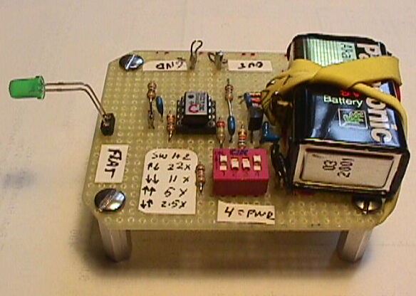
Circuit board setup for testing the green LED.
I worked with Walter Lenk to create a simple current-to-votage circuit board to measure the output of the LEDs.
The power has been turned on with switch-4 and the gain has been set to 22x (220 mV/nA) by setting switch-1 on and switch-2 off. The green LED has been inserted with the flat (cathode) side facing the label FLAT (connected to ground). The output is measured on the opposite side at the GND and OUT terminals.
When measured with a digital multimeter I noticed no noise in the circuit at measurements down to 0.001 V however when the signal is viewed on an oscilloscope 60 cycle hum is present. If the signal is measured with a sampling (rather than integrating) convertor either additional shielding must be used or the 60 cycle signal removed after conversion with digital signal filtering. The whole board could be mounted in and grounded to an aluminum box with the led poking out a hole in the side placed to line up with the exit apeture of the monochrometer.
Schematic
The circuit used a Texas Instruments TCL27L2BCP dual op-amp with the first stage set in a current-to-voltage configuration with a 10 M Ohm feedback resistance and the second stage had gains of 2.5, 5, 11, and 22x.
During the tests the gain for the green LED was set to 22x and the gain for the high-brightness red LED was set to 11x. The effective feedback resistance for the green LED was 2.2 G Ohm and the red 1.1 G Ohm.
Table of experimental data
| wavelength | green led | hi-bright red led |
Monochrometer Output Power (uW) |
green led corrected normalized |
red led corrected normalized |
| 350 | 0.476 | ||||
| 355 | 0.623 | ||||
| 360 | 0.740 | ||||
| 365 | 0.801 | ||||
| 370 | 0.830 | ||||
| 375 | 0.938 | ||||
| 380 | 1.081 | ||||
| 385 | 1.217 | ||||
| 390 | 1.348 | ||||
| 395 | 1.475 | ||||
| 400 | 0.000 | 1.596 | 0.002 | ||
| 405 | 0.001 | 1.735 | 0.016 | ||
| 410 | 0.001 | 1.917 | 0.014 | ||
| 415 | 0.001 | 2.165 | 0.013 | ||
| 420 | 0.002 | 2.472 | 0.022 | ||
| 425 | 0.003 | 2.752 | 0.030 | ||
| 430 | 0.004 | 2.990 | 0.036 | ||
| 435 | 0.004 | 3.189 | 0.034 | ||
| 440 | 0.005 | 3.347 | 0.040 | ||
| 445 | 0.000 | 0.006 | 3.448 | 0.000 | 0.047 |
| 450 | 0.005 | 0.006 | 3.350 | 0.020 | 0.049 |
| 455 | 0.019 | 0.006 | 3.182 | 0.081 | 0.051 |
| 460 | 0.049 | 0.007 | 3.053 | 0.217 | 0.062 |
| 465 | 0.099 | 0.011 | 3.277 | 0.409 | 0.091 |
| 470 | 0.175 | 0.014 | 3.645 | 0.650 | 0.104 |
| 475 | 0.286 | 0.019 | 4.046 | 0.958 | 0.127 |
| 480 | 0.397 | 0.023 | 4.530 | 1.187 | 0.138 |
| 485 | 0.519 | 0.027 | 5.109 | 1.376 | 0.143 |
| 490 | 0.631 | 0.031 | 5.672 | 1.507 | 0.148 |
| 495 | 0.758 | 0.036 | 6.171 | 1.664 | 0.158 |
| 500 | 0.892 | 0.041 | 6.632 | 1.822 | 0.168 |
| 505 | 1.028 | 0.050 | 7.052 | 1.975 | 0.192 |
| 510 | 1.158 | 0.065 | 7.466 | 2.101 | 0.236 |
| 515 | 1.290 | 0.085 | 7.881 | 2.218 | 0.292 |
| 520 | 1.403 | 0.106 | 8.294 | 2.292 | 0.346 |
| 525 | 1.518 | 0.126 | 8.691 | 2.366 | 0.393 |
| 530 | 1.641 | 0.145 | 9.062 | 2.453 | 0.434 |
| 535 | 1.745 | 0.166 | 9.373 | 2.522 | 0.480 |
| 540 | 1.925 | 0.190 | 9.624 | 2.710 | 0.535 |
| 545 | 2.187 | 0.222 | 9.896 | 2.994 | 0.608 |
| 550 | 2.387 | 0.262 | 10.232 | 3.161 | 0.694 |
| 555 | 1.864 | 0.313 | 10.568 | 2.389 | 0.802 |
| 560 | 1.078 | 0.370 | 10.861 | 1.345 | 0.923 |
| 565 | 0.539 | 0.450 | 11.124 | 0.656 | 1.096 |
| 570 | 0.222 | 0.534 | 11.356 | 0.265 | 1.274 |
| 575 | 0.079 | 0.627 | 11.557 | 0.093 | 1.470 |
| 580 | 0.030 | 0.756 | 11.745 | 0.035 | 1.744 |
| 585 | 0.009 | 0.887 | 11.930 | 0.010 | 2.014 |
| 590 | 0.001 | 1.006 | 12.111 | 0.001 | 2.251 |
| 595 | 1.116 | 12.287 | 2.461 | ||
| 600 | 1.180 | 12.457 | 2.567 | ||
| 605 | 1.255 | 12.622 | 2.694 | ||
| 610 | 1.280 | 12.784 | 2.713 | ||
| 615 | 1.323 | 12.940 | 2.770 | ||
| 620 | 1.343 | 13.071 | 2.784 | ||
| 625 | 1.357 | 13.160 | 2.794 | ||
| 630 | 1.367 | 13.225 | 2.801 | ||
| 635 | 1.387 | 13.283 | 2.829 | ||
| 640 | 1.394 | 13.338 | 2.832 | ||
| 645 | 1.406 | 13.385 | 2.846 | ||
| 650 | 1.306 | 13.426 | 2.636 | ||
| 655 | 0.812 | 13.460 | 1.635 | ||
| 660 | 0.403 | 13.488 | 0.810 | ||
| 665 | 0.155 | 13.508 | 0.311 | ||
| 670 | 0.057 | 13.523 | 0.114 | ||
| 675 | 0.016 | 13.534 | 0.032 | ||
| 680 | 0.004 | 13.541 | 0.008 | ||
| 685 | 0.001 | 13.546 | 0.002 | ||
| 690 | 0.000 | 13.548 | 0.000 | ||
| 695 | 13.544 | ||||
| 700 | 13.526 | ||||
| 705 | 13.489 | ||||
| 710 | 13.439 | ||||
| 715 | 13.382 | ||||
| 720 | 13.321 | ||||
| 725 | 13.258 | ||||
| 730 | 13.191 | ||||
| 735 | 13.113 | ||||
| 740 | 12.978 | ||||
| 745 | 12.784 | ||||
| 750 | 12.590 | ||||
| 755 | 12.417 | ||||
| 760 | 12.270 | ||||
| 765 | 12.134 | ||||
| 770 | 11.955 | ||||
| 775 | 11.722 | ||||
| 780 | 11.481 | ||||
| 785 | 11.239 | ||||
| 790 | 10.998 | ||||
| 795 | 10.755 | ||||
| 800 | 10.513 |
References
- Forrest M. Mims III, 1992, Sun photometer with light-emitting diodes as spectrally selective detectors
- HAZE-SPAN, 1998, Haze Sun Photometer Atmospheric Network
- David R. Brooks, 2001, Developoment of an inexpensive hendheld LED-based Sun photometer for the Globe program
- Gregory Garza, 2013, Atmosphere Observation by the Method of LED Sun Photometry
- Forrest M. Mims III, March 2015, Make, Build a Twilight Photometer to Detect Stratospheric Particles